Maple Plots from jh04.1

(This from Math 252 Homework Assignment #04, due Friday February 5th, 1999.)

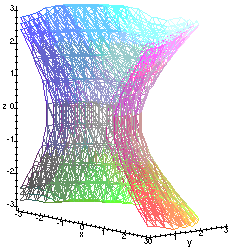
The Maple commands used to produce this plot are as follows:

  with(plots):
  plot1:=implicitplot3d(x^2+y^2-z^2=1,x=-3..3,y=0..3,z=-3..3):
  plot2:=implicitplot3d(x^2+y^2-z^2=2,x=-3..3,y=0..3,z=-3..3):
  plot3:=implicitplot3d(x^2+y^2-z^2=3,x=-3..3,y=0..3,z=-3..3):
  display3d({plot1,plot2,plot3},axes='FRAMED',style='WIREFRAME',
    scaling='CONSTRAINED',orientation=[-40,80]);

Here is the Maple plot of the 3 flow lines, along with the isotimic surfaces, which was asked for in question jh04.1, part 5:

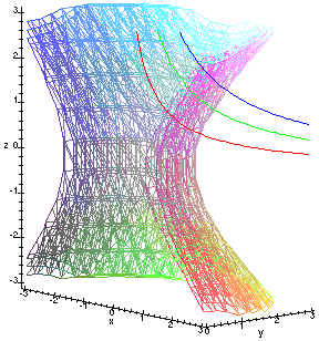
The Maple commands used to produce this plot are as follows:

  with(plots):
  plot1:=implicitplot3d(x^2+y^2-z^2=1,x=-3..3,y=0..3,z=-3..3):
  plot2:=implicitplot3d(x^2+y^2-z^2=2,x=-3..3,y=0..3,z=-3..3):
  plot3:=implicitplot3d(x^2+y^2-z^2=3,x=-3..3,y=0..3,z=-3..3):
  plot4:=spacecurve([t,t,1/t],t=1/3..3,color='RED'):
  plot5:=spacecurve([t,t,2/t],t=2/3..3,color='GREEN'):
  plot6:=spacecurve([t,t,3/t],t=1..3,color='BLUE'):
  display3d({plot1,plot2,plot3,plot3,plot4,plot5,plot6},
    axes='FRAMED',style='WIREFRAME',scaling='CONSTRAINED',
    orientation=[-40,80]);