Maple Plots from jh05.2

(This from Math 252 Homework Assignment #05, due Monday February 15th, 1999.)

Problem jh05.2 asked that the gradient of phi be plotted in Maple. However, the gradient of phi is just the vector field given in problem jh05.1, with the constant a = 0. This will lead to the magnitude of the vector field at (1,0,0) and (-1,0,0) becoming infinite, which may cause plotting problems near these points. In order to avoid this, let's let a = 0.3, which is relatively small but still lets us see qualitative detail.

Using Maple, we have:

  phi:=ln(sqrt(((x-1)^2+y^2+z^2+0.09)/((x+1)^2+y^2+z^2+0.09)));

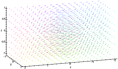
Now if we plot the gradient of this, in Maple, we obtain:

  with(plots):
  gradplot3d(phi,x=-2..2,y=-1..1,z=-1..1,axes='FRAMED',
   arrows='SLIM',grid=[16,8,8],
   orientation=[71,76],scaling='CONSTRAINED');

We can see a field source at (1,0,0) and a field sink at (-1,0,0).

In order to make it clearer, lets consider the field in the xz-plane. Using Maple to substitute y = 0 into phi, one obtains:

  phi_xz:=subs(y=0,phi);

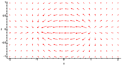
If we then plot the gradient of this field in 2-dimensions, using Maple, we obtain:

  gradplot(phi_xz,x=-2..2,z=-1..1,arrows='SLIM',axes='FRAMED',
    scaling='CONSTRAINED',grid=[20,10],color='RED');

We see that when x = 0, the field lines become parallel, indicating that the divergence is zero on the yz-plane. Therefore, the divergence of the gradient of phi is zero on the yz-plane, and this is just the Laplacian of phi. We can now see why the Laplacian of phi is zero when x = 0.

SFU / Math & Stats / ~hebron / math252 / assignments / sol05 / jh05.2.html

Revised 01 March 1999 by John Hebron.