
Department of Mathematics & Statistics
Fall 2000
MATH 416 - Numerical Analysis II

- e-mail:
- send to class e-mail
Numerical Analysis & Scientific Computing
Traditionally, the subject of numerical analysis is about the design
and analysis of algorithms for solving mathematical equations on a
digital computer. The idea of modern scientific computing, however,
encompasses numerical methodologies as well as issues such as model
development and graphical visualization. The aim of this course is to
discuss numerical techniques for solving differential equations, both
ordinary (ODEs) and partial (PDEs) -- but from a case
study perspective which emphasizes deriving an understanding of
differential equations using computational methods.
outline: initial value ODEs -- linear, nonlinear & systems
boundary value ODEs -- including eigenvalue problems
hyperbolic PDEs -- characteristics & the wave equation
parabolic PDEs -- the diffusion equation
elliptic PDEs -- the Laplace & Poisson equations
special -- integral equations, variational
methods, monte-carlo techniques
texts: Scientific Computing, Michael T Heath, McGraw-Hill 1997
Numerical Analysis, RL Burden & JD Faires, Brooks/Cole 1997 (suggested)
22 November
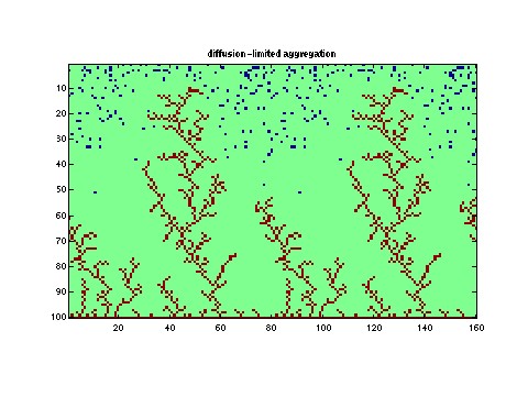
diffusion-limited aggregation script (1K dla.m)

22 November
hw #9 (59K hw09.pdf)
22 November
wave plotting script (1K hw09c.m)
wave data (200K u1.mat)

22 November
random walk script (1K walk.m)
simple random walk script (1K swalk.m)
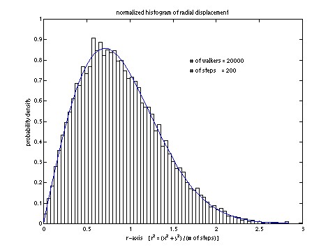
Note, this is not an example of a good graphic, but
rather a hint about what to expect when your code is
behaving well.
17 November
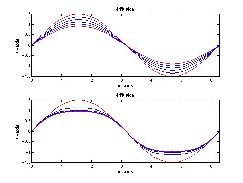
nonlinear diffusion script (1K lect29.m)
X29 ODE function (1K X29.m)

15 November
hw #8 (51K hw08.pdf)
15 November
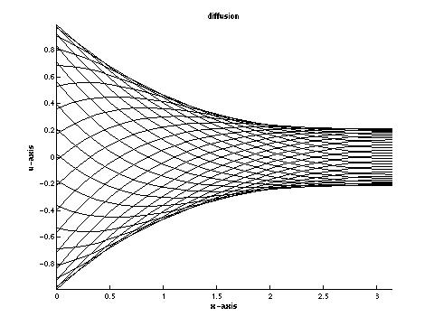
first diffusion script (1K lect28.m)

09 November
homework #7 (45K hw07.pdf)
Lax-Wendroff page (120K page.pdf)
08 November
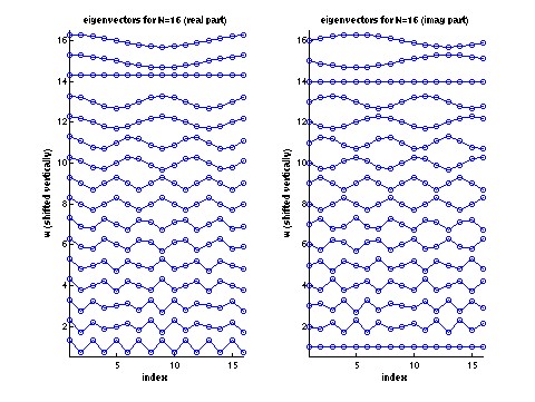
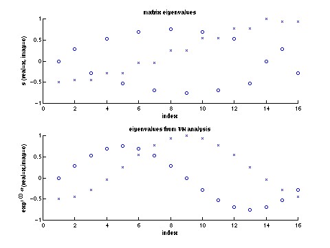
matrix eigenvalue script (1K lect26.m)
leapfrog script (1K lect25.m)
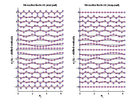
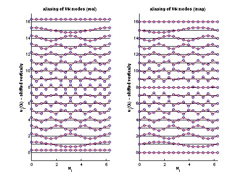
leapfrog VN analysis script (1K lect24.m)


01 November
homework #6 (49K hw06.pdf)
01 November
stability script (1K lect22.m)
error script (1K lect22a.m)

19 October
another one-way wave script (1K lect18.m)

17 October
one-way wave script (1K lect17.m)
derivative script (1K X_1way.m)
12 October
homework #5 (63K hw05.pdf)
stability region script (1K lect16.m)

12 October
matlab ode script (1K lect15.m)
cubic ODE script (1K Xcubic.m)
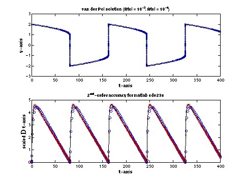
Van der Pol script (1K XvdPol.m)


03 October
homework #4 (49K hw04.pdf)
runge-kutta (RK2) script (1K hw04.m)
03 October
explicit midpoint method (1K lect12z.m)

02 October
HW #3C: consider studying exp(k*cos(x)) for different values of k
29 September
spectral accuracy script (1K lect11b.m)
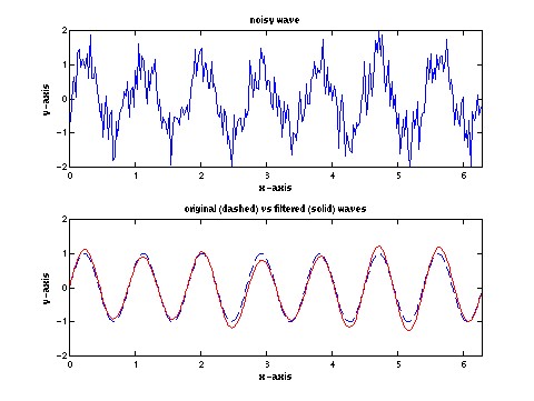
noise filtering script (1K lect11c.m)


28 September
zigzag fft script (1K hw03a.m)
data for 9-point curve (1K data03)
spectral accuracy script (1K lect11.m)
28 September
homework #3 (51K hw03.pdf)
25 September
FFT script (1K lect08.m)

22 September
my homework #0 script (1K hw00c.m)
20 September
homework #2 (49K hw02.pdf)
20 September
newton method BVP script (1K lect07.m)

17 September
HW #1B: note the misplaced solve z1 in the pseudocode (it is changed in the .pdf file above).
HW #1B: verify the second-order convergence of your code.
HW #1Cii: check the conditioning of the matrix.
17 September
homework #1 (49K hw01.pdf)
11 September
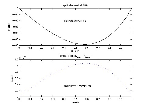
BVP plotting script (1K lect03.m)
06 September
first lecture, room AQ 5020, 10:30am
syllabus (57K pdf)
student info sheet (33K pdf)
homework #0 (51K pdf)
matlab plotting script (1K hw00a.m)
matlab recursion script (1K hw00b.m)
40 page matlab primer (279K pdf)
download adobe (reader)
06 September
a scientific computing example: snell's law (code9a.m)
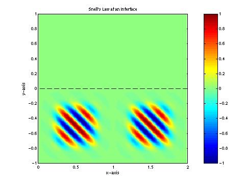
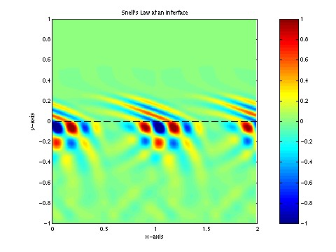

Numerical solution of the 2D wave equation with a Snell's
Law interface (y=0) marked by the dashed line. Three times are shown:
initial time (top), interface interaction (mid), and final time (bot).
The wavespeed above the interface is half of the value below. The
domain is horizontally-periodic in x, and two periods are shown in
each panel. The initial wavepacket is designed to travel at 45
degrees to the interface (this is adjustable in the matlab script).
Note the interference pattern formed by the incident and reflected
waves below the interface in the mid-panel. By the final time, the
reflected wavepacket has cleared the interface and is heading (angle
of reflection should be -45 degrees) towards the Dirichlet lower
boundary. Since the upper wavespeed is smaller, the transmitted wave
has shorter wavelength and travels at a larger angle (~69.3 degrees)
from the interface.